Nearly two years ago, the Binder Project released the beta version
of BinderHub, the technology behind mybinder.org. Since then, mybinder.org has grown to serve nearly 90,000 launches each week and hit the two million launches in a year milestone last year. Over these two years BinderHub has matured as technology and community. Several new organizations now run their own BinderHubs and have joined the community of maintainers.

Today we are proud to announce that we’ve removed the “beta” label from all pages served by BinderHub. BinderHub is now a tool with a track record of working well in production (both at mybinder.org and in other deployments), its general features and API have stabilized, and JupyterHub, the underlying technology that BinderHub uses, is close to its 1.0 release.

A big thank you to all those who have used, commented, advocated, advertised, contributed, maintained and funded this journey. The deployment at mybinder.org is funded with grants from the Moore Foundation and the Google Cloud Platform.

Who else has deployed a BinderHub?

A goal of Project Binder is to build modular, open-source tools that
others can deploy for their own communities. BinderHub, the core technology behind mybinder.org, runs on Kubernetes this means it can be deployed on many cloud providers or even on your own hardware. Over the years, we have seen many new organizations deploy their own BinderHubs. Here are our highlights of other organizations who have joined the BinderHub community.

GESIS were the first to deploy a public BinderHub that is operated independently of mybinder.org. The GESIS BinderHub instance went live
in December 2017 and has been running ever since. They are frequent
contributors to the upstream project. Their BinderHub runs on a bare metal
Kubernetes cluster.

The Pangeo Project instance was the next to come online, launching their
public BinderHub instance in September 2018 (more details in their blog post). They provide additional compute resources and have customized their setup to provide on-demand dask clusters to users. Try out one
of their examples using ocean data. The Pangeo cluster is hosted on Google Kubernetes Engine.

Recently, the Turing Way project has been working on deploying a BinderHub at the Turing Institute in the UK. This BinderHub will serve both internal and external users with the goal of making it easier to share data science projects. They have run several workshops including one that teaches scientists and research software engineers how to deploy their own BinderHub instance. Recently they led a workshop in which ten academics and IT staff deployed their own BinderHub on the Microsoft Azure cloud! Sarah Gibson from their team has recently joined the team that operates mybinder.org.

Finally, the Pacific Institute for the Mathematical Sciences (PIMS) runs a service called Syzygy. It deploys several JupyterHubs and BinderHubs for scientific organizations around Canada. A Binder team recently held a tutorial on deploying Binder and JupyterHub at the PEARC (you can find slides for the talk here). They have also provided a script for deploying JupyterHub (and Binder) on Terraform.

What’s next?

Now that BinderHub is not in beta anymore, what is next? As Project Binder we will focus on adoption, training, and growing the Binder community. This means growing the creation of Binder-ready repositories (repositories that have the necessary structure for Binder to create the environment needed to run the repository’s code). We will increase our outreach and marketing efforts to make sure a diverse audience everywhere around the world knows about Binder.

We will also work on making it easier to setup and operate a public BinderHub no matter what cloud vendor you are using. We are excited to see more organizations deploy their own BinderHubs for their communities. In the coming months, our goal is to create a federation of public BinderHubs
that operate in unison to serve the global user base of mybinder.org.

If this caught your attention consider joining the Binder community, or contributing to Project Binder! A good place to start is the Jupyter Community Forum or dive straight into the code on GitHub.

BinderHub is out of Beta! was originally published in Jupyter Blog on Medium, where people are continuing the conversation by highlighting and responding to this story.

We have some exciting news to share regarding the Jupyter Server Design and Roadmap Workshop as part of the Jupyter Community Workshop series funded by Bloomberg. This workshop will take place May 16th and 17th just outside Paris France at the IBM facility in Bois-Colombes.

Jupyter Notebook has proven to be a tremendous tool in the scientific and analytic computing spaces. It is widely used at universities and businesses alike, enabling the ability to interactively analyze and view data in various ways, quickly and easily. However, as computational capabilities improve, the need to move Notebook kernels closer to the compute resources also increases. As a result, new requirements for how a given solution is configured and deployed are introduced.

The Jupyter Server Design and Roadmap Workshop will focus on how we can bring together what has been learned over the years to address the needs of future environments, while clearly defining the separation between client and server. Items that will be discussed include:

1. What aspects of the current Jupyter Notebook framework should be considered as “the server”?

2. How will extensions be exposed and consumed?

3. Backwards compatibility is important. How can we move forward while retaining current capabilities?

4. How can we introduce the ability for others to provide kernel-deployment frameworks of their own and how those frameworks are discovered?

5. Basic improvements that bring the server up to date (e.g., async/await — particularly in kernel life-cycle management)

6. General multi-tenancy capabilities will be explored such that the server can serve more than just a single client.

7. How to convey kernel-specific parameters from the client, thru the server, to the kernel launch framework?

Should you be interested in joining us for this workshop, please fill out this Google Form. Space is limited.

Acknowledgements

We’d like to acknowledge Bloomberg for their generous support in making this workshop, and the entire series, possible. Thank you!

We’d also like to thank IBM for providing the facility and hosting the Jupyter Server Design and Roadmap Workshop.

Jupyter Community Workshop: Jupyter Server Design and Roadmap Workshop was originally published in Jupyter Blog on Medium, where people are continuing the conversation by highlighting and responding to this story.

Today, we are pleased to announce the 1.0 release of JupyterHub. We’ve come a long way since our first release in March, 2015. There are loads of new features and improvements covered in the changelog, but we’ll cover a few of the highlights here.

You can upgrade jupyterhub with conda or pip:

(Before upgrading, always make sure to backup your database!)

conda install -c conda-forge jupyterhub==1.0.*
pip install --upgrade jupyterhub==1.0.*

UI for named servers

Named servers are a concept in JupyterHub that allows each user to have more than one server (e.g. a ‘gpu’ server with access to gpus, or a ‘cs284’ server with the necessary resources for a given class). JupyterHub 1.0 introduces UI for managing these servers, so users can create/start/stop/delete their servers from the hub home page:

Improved pending spawn handling and less implicit spawn behavior

When users launch their server, they will be faced with a progress bar showing the progress. Spawners can emit custom messages to indicate the stages of launch, which are especially useful when it can take a while.

Support for total internal encryption with SSL

If your JupyterHub is publicly accessible, we hope you are using HTTPS (it’s never been easier, thanks to letsencrypt)! However, JupyterHub exclusively used HTTP for internal communication. This is usually fine, especially for single-machines, but for deployments on distributed or shared infrastructure it’s a good idea to encrypt communication between your components. With 1.0, you can enable SSL encryption and authentication of all internal communication as well. Spawners must support this feature by defining Spawner.move_certs. Currently, local spawners and DockerSpawner support internal ssl.

Support for checking and refreshing authentication

JupyterHub authentication is most often managed by an external authority, e.g. GitHub OAuth. Auth state can be used to persist credentials, such as enabling push access to repositories or access to resources. These credentials can sometimes expire or need refreshing. Until now, expiring or refreshing authentication was not well supported by JupyterHub. 1.0 introduces new configuration to refresh or expire authentication info:

c.Authenticator.auth_refresh_age allows authentication to expire after a number of seconds.

c.Authenticator.refresh_pre_spawn forces a refresh of authentication prior to spawning a server, effectively requiring a user to have up-to-date authentication when they start their server, which can be important when the user environment should have credentials with access to external resources.

Authenticator.refresh_auth defines what it means to refresh authentication (default is nothing, but can check with external authorities to re-load info such as tokens or group membership) and can be customized by Authenticator implementations.

Thanks!

Huge thanks to the many people who have contributed to this release, whether it was through discussion, testing, documentation, or development.

Announcing JupyterHub 1.0 was originally published in Jupyter Blog on Medium, where people are continuing the conversation by highlighting and responding to this story.

The University of Edinburgh is happy to announce our upcoming event as part of the Jupyter Community Workshop series funded by Bloomberg. The University will be hosting a three-day event, the core aspect of this event being a hackathon focused on adding improvements, fixes and extra documentation for the nbgrader extension. Alongside this we will also hold an afternoon of talks highlighting how Jupyter can be used in education at varying levels. The event will take place on 29 to 31 May at the University of Edinburgh, with the afternoon of talks taking place on 30 May.

The first and main part of the event will be the nb grader hackathon. nbgrader is a Jupyter extension that allows for the creation and marking of notebook-based assignments. Here at the University, we have adopted nbgrader and our developers have integrated the extension into our Jupyter service Noteable. The hackathon will focus on improving the core features and extending the abilities of nbgrader; by adding such features, it will be easier for institutions to adopt and embed both Jupyter and nbgrader into their teaching practice.

The second, equally important part of our event is a series of talks aimed at highlighting the uses of Jupyter within education. As part of developing our local Jupyter service, we have uncovered many use cases across the University of how Jupyter can be adopted in a variety of disciplines and scenarios that we are keen to share. We will also be able to showcase an institutional approach to adopting and supporting Jupyter at scale. On top of this, there is also the opportunity to hear from many of our hackathon attendees. This series of talks is aimed at academic colleagues, and teaching and support staff at any level of education and includes an evening networking event to allow attendees to further explore how they may introduce Jupyter to their institution.

What are we working on?

We have worked with our local developers and scoured the nbgrader Github repo to devise a plan of attack for the hackathon in terms of features and improvement. We’re keen to engage with the wider community regarding these goals and have created a post on the Jupyter Discourse to allow further discussion.

• Support for Multiple course/Multiple classes. Instructors that teach multiple course using nbgrader or students enrolled on multiple course. Multiple Courses (ref: PR #1040) vs Support for multiple classes via Jupyterhub groups (PR #893)
• Considerations for LTI use: Users/Courses not in the database at startup
• Support for Multiple markers for one assignment (part of issue #1030, which extends #998)
• API Tests have hard-coded file copy methods to pre-load the system to enable testing, and os.file_exists-type tests for release & submit tests
• Generation of feedback copies for students within the formgrader UI (to mirror the existing terminal command). Also consider ability to disseminate this feedback back to students within nbgrader.

Want to get involved?

If you would like to be involved in the hackathon, we still have an amount of funding left for travel and accommodation. We are looking for participants who have a good understanding of Jupyter and nbgrader who would be able to attend all three days of the event. If you would be able to attend, please complete the following form: [https://edin.ac/2vP8bFS].

If you can’t attend but want to have a say on what is worked on during the hackathon then join the discussion on the Jupyter Discourse (if you’re new to Jupyter this is an excellent place to head to for community discussions)

If you’d like to come along to our Jupyter community afternoon on 30 May, book a place via Eventbrite.

University of Edinburgh Jupyter Community nbgrader Hackathon was originally published in Jupyter Blog on Medium, where people are continuing the conversation by highlighting and responding to this story.

I would like to share some exciting news about a Jupyter Community Workshop in South America!

The workshop will be held in Córdoba, Argentina, from Jun 22nd to Jun 23rd, 2019. The event is being hosted in the Quorum Convention Center, in the heart of one of the more prominent technological areas in Córdoba (Ciudad Empresaria).

In this two-day event, there will be hands-on discussions, hacking sessions, and technical presentations, with Jupyter developers and South American open source contributors and Jupyter users, with the ultimate goal to create and foster a core of South American Jupyter contributors.

Thanks to the generous support provided by Bloomberg, we have funds to support the attendance of people from South America. If you are interested in joining us for this workshop, please complete the interest form.

Note that the deadline is June 3rd (just one week ahead), so don’t delay in completing form!

Spanish (short version ;-)

El 22 y 23 de Junio de 2019, en la Ciudad de Córdoba, se llevará a cabo un taller para fomentar el desarrollo de una Comunidad Sudamericana de contribuyentes al Project Jupyter. Gracias a Bloomberg, tenemos fondos para solventar tu participación en el taller. Si estás interesado en participar, no dudes en llenar la siguiente forma. Estará abierta sólo hasta el 3 de Junio, así que no te duermas!

Portuguese (short version ;-)

Nos dias 22 e 23 de junho de 2019, na cidade de Córdoba, será realizado um workshop para promover o desenvolvimento de uma comunidade sul-americana de colaboradores do Project Jupyter. Graças à Bloomberg, temos fundos para pagar sua participação no workshop. Se você está interessado em participar, não hesite em preencher o seguinte formulário. Será aberto apenas até 3 de junho, então não deixe pra mais tarde!

Why a Workshop for South American contributors?

The Jupyter community is the vital force that builds and sustains the Jupyter ecosystem. In our workshop, we will begin building an active South American Jupyter community of contributors. This will greatly increase the diversity of our current Jupyter community, bringing not only new ideas but also new Jupyter developments and solutions to solve some of the problems we see in this part of the world.

We will start this process with an event bringing people from various areas of South America to Córdoba, Argentina to work/sprint/discuss some of the pieces of the Jupyter ecosystem. Our ultimate plan is to plant seeds to disseminate the Jupyter Ecosystem in different regions of South America, accelerating the South American Jupyter community growth.

Acknowledgements

This event would not have been possible without the generous support provided by Bloomberg, who made this workshop series possible.

Jupyter Community Workshop: South America was originally published in Jupyter Blog on Medium, where people are continuing the conversation by highlighting and responding to this story.

The problem

We love Jupyter notebooks for accommodating a computational narrative — a combination of explanation, code, and the output of this code.
Unfortunately, some tasks cannot be accomplished well by notebooks.
If you are writing documentation for your software project, chances are that you want to provide navigation across many tutorials and explanation pages.
You will also want to automatically document the API, perhaps also maintain a bibliography, and you certainly will want all the classes and functions from your module to automatically link to their documentation pages.
In short, your best bet is Sphinx.

Sphinx does not provide a way to build a computational narrative: by itself, it cannot execute any code, nor does it know how to handle the output of that code. This limitation is well known and there are great tools offering a workaround; I’ll list the ones that I know about:

• nbsphinx allows incorporating executed notebooks into a documentation website. Unfortunately, markdown used in notebooks is a much more limited markup language than restructured text.
• sphinx-gallery takes a collection of scripts, executes them, shows the code and the output in the documentation, and even automatically links object names occurring in a script to their documentation. It also parses rst-formatted comments and renders those.

Jupyter-sphinx

We have just made an addition to this list, a freshly rewritten jupyter-sphinx extension, that was previously specialized to render Jupyter widgets.
To embed arbitrary output in your documentation using jupyter-sphinx you only need to use the jupyter-execute directive:

.. jupyter-execute::

  print('Hello world!')

Under the hood, all such code chunks are converted to cells in a notebook and executed using nbconvert. We then rely on the Jupyter format and protocol to interpret what to do with the results of executing the code. This means you already know how the output will be shown: we apply exactly the same logic as Jupyter notebook does.

For example, here we make a plot:

And here we are rendering some widgets:

If you want to see jupyter-sphinx used to make package documentation, check out adaptive, the first adopter (full disclosure—I am one of its authors).

An important corollary: building upon the Jupyter kernel protocol makes jupyter-sphinx language-agnostic; jupyter-sphinx works with absolutely any language for which a kernel exists.

Try it

We have freshly published a release candidate, give it a go using pip install jupyter-sphinx==0.2.0rc1 --pre. We would love to hear your feedback, especially if you are using other ways of embedding outputs in the documentation, or if you are using an older version of jupyter-sphinx.

Integrating output in documentation with jupyter-sphinx was originally published in Jupyter Blog on Medium, where people are continuing the conversation by highlighting and responding to this story.

… from Jupyter notebooks to standalone applications and dashboards

The goal of Project Jupyter is to improve the workflows of researchers, educators, scientists, and other practitioners of scientific computing, from the exploratory phase of their work to the communication of the results.

But interactive notebooks are not the best communication tool for all audiences. While they have proven invaluable to provide a narrative alongside the source, they are not ideal to address non-technical readers, who may be put off by the presence of code cells, or the need to run the notebook to see the results. Finally, following the order as the code often results in the most interesting content to be at the end of the document.

Another challenge with sharing notebooks is the security model. How can we offer the interactivity of a notebook making use of e.g. Jupyter widgets without allowing arbitrary code execution by the end user?

We set ourselves to solve these challenges, and we are happy to announce the first release of voilà.

Voilà turns Jupyter notebooks in standalone web applications.

• Voilà supports Jupyter interactive widgets, including the roundtrips to the kernel.
• Voilà does not permit arbitrary code execution by consumers of dashboards.
• Built upon Jupyter standard protocols and file formats, voilà works with any Jupyter kernel (C++, Python, Julia), making it a language-agnostic dashboarding system.
• Voilà is extensible. It includes a flexible template system to produce rich application layouts.

Installation and first-time use

Voilà can be installed from pypi:

pip install voila

or conda-forge:

conda install voila -c conda-forge

Upon installation, several components are installed, one of which is the voila command-line utility. You can try it by typing voila notebook.ipynb. It results in the browser opening to a new tornado application showing markdown cells, rich outputs, and interactive widgets.

As you can see in the screencast, Jupyter interactive widgets remain fully functional even when they require computation by the kernel.

You can immediately try out some of the command-line options to voilà

• with --strip_sources=False, input cells will be included in the resulting web application (as read-only pygment snippets).
• with --theme=dark, voilà will make use of the dark JupyterLab theme, which will apply to code cells, widgets and all other visible components.

Note that code is only shown, voilà does not allow users to edit or execute arbitrary code.

Voilà's execution model

The execution model of voilà is the following: upon connection to a notebook URL, voilà launches the kernel for that notebook, and runs all the cells as it populates the notebook model with the outputs.

After the execution, the associated kernel is not shut down. The notebook is converted to HTML and served to the user. The rendered HTML includes JavaScript that establishes a connection to the kernel. Jupyter interactive widgets referred in cell outputs are rendered and connected to their counterpart in the kernel. The kernel is only shut down when the user closes their browser tab.

The current version of voilà only responds to the initial GET request when all the cells have finished running, which may take a long time, but there is ongoing work on enabling progressive rendering, which should make it into a release soon.

An important aspect of this execution model is that the front-end does not determine what code is run by the backend. In fact, unless specified otherwise (with option --strip-sources=False), the source of the rendered notebook does not even make it to the front-end. The instance of the jupyter_server instantiated by voilà actually disallows execute requests by default.

Support for custom interactive widgets

Voilà can render custom Jupyter widget libraries, including (but not limited to) bqplot, ipyleafet, ipyvolume, ipympl, ipysheet, plotly, ipywebrtc, etc.

Together with ipympl, voilà is actually a simple means to render interactive matplotlib figures in a standalone web application:

Voilà is language-agnostic

Voilà can be used to produce applications with any Jupyter kernel. The following screencast shows how voilà can be used to produce a simple dashboard in C++ making use of leaflet.js maps, with the xeus-cling C++ kernel and the xleaflet package.

We hope that voilà will be a stimulant to other languages (R, Julia, JVM/Java) to provide stronger widgets support.

Richer layouts with Voilà templates

The main extension point to voilà is the custom template system. The HTML served to the end-user is produced from the notebook model by applying a Jinja template, which can be defined by the user.

An example template for voilà is the voila-gridstack template, which can be installed from pypi with

pip install voila-gridstack

You can try it by typing voila notebook.ipynb --template=gridstack.

The gridstack voilà template makes use of the cell metadata to lay out the application.

A roadmap item for the gridstack voilà template is to support the entire spec for the deprecated jupyter dashboards and to create a WYSIWYG editor for these templates in the form of a JupyterLab extension.

Note that voila-gridstack template is still at an early stage of development.

How to make custom voilà templates?

A voilà template is actually a folder placed in the standard directoryPREFIX/share/jupyter/voila/templates and which may include

• nbconvert templates (the jinja templates used to transform the notebook into HTML)
• static resources
• custom tornado templates such as 404.html etc.

All of these are optional. It may also contain a conf.json file to set up which template to use as a base. The directory structure for a voilà template is the following:

PREFIX/share/jupyter/voila/templates/template_name/
|
├── conf.json                # Template configuration file
├── nbconvert_templates/     # Custom nbconvert templates
├── static/                  # Static directory
└── templates/               # Custom tornado templates

The voilà template system can be used to completely override the behavior of the front-end. One can make use of modern JavaScript frameworks such as React or Vue.js to produce modern UI including Jupyter widgets and outputs.

Another example template for voilà is voila-vuetify, which is built upon vue.js:

The voila-gridstack and voila-vuetify templates are still at an early stage of development, but will be iterated upon quickly in the next weeks as we are exploring templates.

A Jupyter server extension

Beyond the voila command-line utility, the voilà package also include a Jupyter server extension, so that voilà dashboards can be served alongside the Jupyter notebook application.

When voilà is installed, a running Jupyter server will serve the voilà web application under BASE_URL/voila.

The Jupyter Community Workshop on Dashboarding

From June 3rd to June 6th 2019, a community workshop on dashboarding with Project Jupyter took place in Paris. Over thirty Jupyter contributors and community members gathered to discuss dashboarding technologies and hack together.

Several dashboarding solutions such as Dash and Panel were presented during the workshop and featured at the PyData Paris Meetup which was organized on the same week.

The workshop was also the occasion for several contributors to start working on voilà. Custom templates, a dashboard gallery, logos and UX mockups for JupyterLab extensions have been developed.

We will soon publish a more detailed post on the workshop, detailing the many tracks of development that have been explored!

What is coming?

There is a lot of planned work around voilà in the next weeks and months. Current work streams include better integration with JupyterHub for publicly sharing dashboard between users, as well as JupyterLab extensions (a voilà "preview" extension for notebooks, and a WYSIWYG editor for dashboard layouts). There are also ongoing discussions with the OVH cloud provider (which already supports binder by handling some of its traffic) on hosting a binder-like service dedicated to voilà dashboards. So stay tuned for more exciting developments!

Last but not least, we are especially excited about what you will be building upon voilà!

Acknowledgments

The development of voilà and related packages at QuantStack is sponsored by Bloomberg.

We are also grateful to the attendees of the Jupyter Community Workshop on Dashboarding for their numerous contributions to voilà!

We would like to thank Chris Holdgraf for his work on improving documentation, and integration with JupyterHub.

We should mention Yuvi Panda and Pascal Bugnion for getting the voila-galleryproject off the ground during the workshop. We are grateful to Zach Sailer for his continued work on improvingjupyter_server. We should finally not forget to mention the prior art by Pascal Bugnion with the Jupyter widgets server which was also an inspiration for voilà.

About the Authors

Sylvain Corlay is the founder and CEO of QuantStack and a core team member for Project Jupyter.

Maarten Breddels is an independent scientific software developer partnering with QuantStack on numerous projects, and a core developer of Project Jupyter.

And voilà! was originally published in Jupyter Blog on Medium, where people are continuing the conversation by highlighting and responding to this story.

Whenever someone says ‘You can do that with an extension’ in the Jupyter ecosystem, it is often not clear what kind of extension they are talking about. The Jupyter ecosystem is very modular and extensible, so there are lots of ways to extend it. This blog post aims to provide a quick summary of the most common ways to extend Jupyter, and links to help you explore the extension ecosystem.

JupyterLab extensions (labextension)

JupyterLab is a popular ‘new’ interface for working with Jupyter Notebooks. It is an interactive development environment for working with notebooks, code and data — and hence extremely extensible. Using JupyterLab extensions, you can add entirely new functionality or change almost any aspect of how the interface behaves. These are written in TypeScript or JavaScript, and run in the browser.

The JupyterLab documentation has information on how to install & use extensions, as well as how to author & distribute them. You can also discover extensions by searching on GitHub or npmjs.com

My favorite JupyterLab extension is jupyterlab-vim — it lets you fully use Vim keybindings inside JupyterLab!

Classic Notebook extensions (nbextension)

When people think of ‘the notebook interface’, they are probably thinking of the classic Jupyter Notebook. You can extend any aspect of the notebook user experience with nbextensions. These are little bits of client-side JavaScript that allow you to add / change functionality as you wish. They are the Classic Notebook equivalent to JupyterLab extensions.

The Jupyter Notebook documentation has information on how to install or develop extensions. The Unofficial Jupyter Notebook extensions repository has a lot of popular extensions and a GUI extension manager you can use to install nbextensions.

My favorite nbextension provides a collapsible Table of Contents for your notebooks.

Notebook Server Extensions (serverextension)

Unlike JupyterLab or nbextensions, Jupyter Notebook Server extensions are written in Python to add some serverside functionality. There are two primary use cases for server extensions.

The first use case is to provide a backend for a particular JupyterLab or classic notebook extension. An example is the jupyterlab-latex JupyterLab extension, which provides live previews of LaTeX files in JupyterLab. It has a frontend JupyterLab extension to integrate with the JupyterLab text editor, and a backend serverextension component that actually runs the LaTeX commands to produce the output displayed to you.

The second use case is to provide any user interface backed by any kind of server side processing. Server extensions can function as arbitrary Tornado HTTP handlers — so any web application you can think of, you can write as a Jupyter serverextension. An example is nbgitpuller, which provides UI and mechanisms to distribute notebooks from git repositories to your users in a transparent way.

My favorite here is jupyter-rsession-proxy, which lets you run RStudio in JupyterHub environments!

Jupyter Kernels

You might be most familiar with using Jupyter notebooks with Python, but you can use a ton of other languages when writing your notebook: R, Julia, JavaScript, Octave, Scala/Spark, interactive C++, bash, or even Matlab! These are called kernels, and they speak the language agnostic Jupyter protocol over zeromq. You can write a new kernel for your language by directly implementing the Jupyter protocol, by wrapping it with the metakernel project, or using C++ bindings via Xeus. Once a kernel exists, it seamlessly works with any Jupyter frontend — classic notebook, JupyterLab, nteract, the terminal jupyter console, the graphical Qt Console , etc.

My favorite kernel is the linux kernel.

IPython Magics

If you’ve written %matplotlib inlinein a notebook, you have used an IPython magic. These are almost like macros for Python — you can write custom code that parses the rest of the line (or cell), and do whatever it is that you want.

Line magics start with one % symbol and take some action based on the rest of the line. For example, %cd somedirectory changes the current directory of the python process. Cell magics start with %% and operate on the entire cell contents after it. %%timeit is probably the most famous – it’ll run the code a number of times and report stats on how long it takes to run.

You can also build your own magic command that integrates with IPython. For example, the ipython-sql package provides the%%sql magic command for working seamlessly with databases. However, remember that in contrast to the extensions listed so far, IPython magics only work with the IPython kernel.

My favorite use of IPython magics is this blog post by Matthias Bussonnier, which makes great use of custom magics to seamlessly integrate Python, R, C and Julia in the same notebook.

IPython Widgets (ipywidgets)

IPython Widgets (ipywidgets) provide interactive GUI widgets for Jupyter notebooks and the IPython kernel. They let you and the people you share your notebooks with explore various options in your code with GUI elements rather than having to modify code. Coupled with something like voila, you can make dashboard-like applications for other people to consume without realizing it was created completely with a Jupyter Notebook!

You can build your own custom widgets to provide domain-specific interactive visualizations. For example, you can interactively visualize maps with ipyleaflet, use itk-jupyter-widget to explore image segmentation/registration problems interactively, or model 3D objects with pythreejs.

Check out the vdom project for a more reactive take on the same problem space, and xwidgets for a C++ implementation

Contents Manager

Whenever you open or save a notebook or file through the web interface, a ContentsManager decides what actually happens. By default it loads and saves files from the local filesystem, but a custom contents manager could do whatever it wants. A popular use case it to load/save contents from somewhere other than the local filesystem — Amazon S3 / Google Cloud Storage, PostgreSQL, HDFS, etc. When using one of these, you can load / save notebooks & files via the web interface as if they are on your local filesystem! This is extremely useful if you are already using any of these to store your data.

My favorite contents manager is Jupytext. It does some magic during save/load to give you a .py equivalent of your .ipynb, and keeps them in sync. You can explore code interactively in your notebook, then open the .py file in an IDE to do some heavy text editing, and automatically get all your changes back in your notebook when you open it again. It’s quite magical.

Extending JupyterHub

JupyterHub is a multi-user application for spawning notebooks & other interactive web applications, designed for use in classrooms, research labs and companies. These organizations probably have other systems they are using, and JupyterHub needs to integrate strongly with them. Here is a non-exhaustive list of ways JupyterHub can be extended.

Authenticators

JupyterHub is a multi-user application, so users need to log in somehow — ideally the same way they log in to every other application in their organization. The authenticator is responsible for this. Authenticators already exist for many popular authentication services — LDAP, OAuth (Google, GitHub, CILogon, Globus, Okta, Canvas, etc), most LMS with LTI , SAML, JWT, plain usernames & passwords, linux users, etc. You can write your own or customize one that exists very easily, so whatever your authentication needs — JupyterHub has you covered.

Spawners

Using pluggable spawners, you can start a Jupyter Notebook Server for each user in many different ways. You might want them to spawn on a node with docker containers, scale them out with Kubernetes, use it on your HPC cluster, have them run along your Hadoop / Spark cluster, contain them with systemd, simply run them as different linux users or in many other possible ways. The spawners themselves are usually extremely configurable, and of course you can write your own.

Services

Often you want to provide additional services to your JupyterHub users — cull their servers when idle, or allow them to publish shareable notebooks. You can run a JupyterHub service to provide these — or similar — services. Users can make requests to them with their JupyterHub identities, and the services can make API calls to JupyterHub too. These can be arbitrary processes or web services — BinderHub is implemented as a JupyterHub service, for example.

NBConvert Exporter

nbconvert converts between the notebook format and various other formats — if you’ve exported your notebook to PDF, LaTeX, HTML, or used nbviewer, you have used nbconvert. It has an exporter for each format it exports to, and you can write your own to export to a new format — or to just massively customize an existing export format. If you’re performing complex conversion operations involving notebooks, you might find writing an exporter to be the cleanest way to accomplish your goals.

My happiest moment when researching for this blog post is finding out that a docx exporter exists.

Bundler Extensions

Bundler extensions let you add entries to the Download as item in the menu bar. They are often paired with an nbconvert exporter to make the exporter more discoverable, though you can also write a custom bundler extension to do any kind of custom processing of a notebook before downloading. For example, nbreport provides a bundler extension that cleans up the notebook in a way suitable for viewing as a report & exports it as HTML.

Repo2Docker

repo2docker turns git (and other) repositories into reproducible, data science focused docker images. mybinder.org (and other binderhub installations) rely on it to build and launch interactive Jupyter/RStudio sessions from git repositories. There are currently two ways to extend repo2docker.

BuildPacks

repo2docker looks at the contents of the repository to decide how to build it. For example, if there is a requirements.txt it sets up a miniconda environment to install python packages into, while if there is an install.R file it makes sure R/RStudio is installed. Writing a new BuildPack lets you extend this behavior to add support for your favorite language, or customize how an existing language is built.

ContentProviders

The repo part of repo2docker is a misnomer — you can turn anything into a docker image. Currently, it supports git, local folder and zenodo repositories — but you can add support for your favorite source of reproducible code by making a new ContentProvider!

Is that all?

Of course not? The Jupyter ecosystem is vast, and no one blog post can cover them all. This blog post is already missing a few — enterprise gateway, TLJH Plugins, etc. As time marches on, there will be newer components and newer ways of extending things that have not even been imagined yet. Leave a comment about what else is missing here.

Look forward to seeing what kinda beautiful extensions y’all create!

99 ways to extend the Jupyter ecosystem was originally published in Jupyter Blog on Medium, where people are continuing the conversation by highlighting and responding to this story.

Binder + Zenodo: A how-to guide

Interactive and reproducible repositories powered by Zenodo and Binder.

When the Binder project was first launched, we imagined a world in which scientific scholarship and reproducibility could be carried out by the community using a fully-open stack of technology. We’re happy to say that this is now possible!

The BinderHub team recently added in support for building Binder links that point to Zenodo repositories. Zenodo is a general purpose open-access repository hosted by CERN that allows researchers to archive and apply a DOI to information that they put up on the web.

Zenodo has the ability to archive GitHub repositories, which means that you can archive the code, data, or reports that underly a scientific analysis and assign it a unique, citeable identifier. Now that BinderHub knows how to resolve a Zenodo identifier, you’ll be able to share Binder links that point to Zenodo and provide interactive access to your repository, letting readers reproduce results and interact with your analyses!

Here’s a quick primer for how to do this:

Step 1: Create a Zenodo account

First off you’ll need to create an account on Zenodo. You can
do so using a number of different log-in options.

Step 2: Create your Binder-ready repository on GitHub

Next, you should create your Binder-ready repository on GitHub. Binder uses pre-existing best practices in data science in order to infer and build the environment needed for your repository.

To make a repository Binder-ready, follow the instructions in the Binder docs.
Briefly, what you need to do is add the configuration files that define the environment needed to run your code. Once those files are in place, and you’ve added an analysis script (a Jupyter or R Notebook) that actually runs your code and displays the results, your repository is ready to build with Binder.

Step 3: Make sure your repository is ready to be published!

Once you create a DOI for your repository, it will be frozen in time — you won’t be able to easily update it. So double check that the repository builds properly with Binder and runs the way that you’d expect it to.

Make sure to launch a Binder from your repository and run the analyses you’d like others to run. If they produce the expected result from within a Binder session, then they’ll continue to do so for others (assuming you have pinned your versions and followed other best practices in reproducibility).

Step 4: Create a Zenodo DOI for your repository

Now that your repository is ready, you’ll connect Zenodo with GitHub to create a DOI for your repository. Remember that this will be unique to the current state of the repo — future changes to this repository won’t be reflected in the DOI.

We recommend following the GitHub Citable Code Guide which provides some best-practices for creating your Zenodo DOI for a GitHub repository. Click the image below to be taken to this (excellent) guide.

Once you’re done, you should have a Zenodo DOI badge
like the one below:

Step 5: Create a Binder link for your Zenodo DOI

Finally, use your Zenodo DOI to create a Binder link that allows others to interact with and replicate your results. You can create a Binder link for your Zenodo record by heading to https://mybinder.org and filling in the form:

This will give you a link you can share with others as well as the Markdown and reStructured text snippets for creating a badge.

The link’s structure should look like this:

https://mybinder.org/v2/zenodo/<zenodo-DOI>

For example, if your Zenodo DOI is 10.5281/zenodo.3242074 (corresponding to this zenodo repository), the Binder link for it would be:

https://mybinder.org/v2/zenodo/10.5281/zenodo.3242074/

You can even pair this Binder link with your Zenodo DOI badge that
we showed above!

And that’s it! You now have an archived version of your analysis with a unique identifier. This identifier can be used in conjunction with BinderHub to allow readers to interact with your code and results!

Last minute update 🎉

A few hours before publishing this post we merged a contribution from Tom Morrell who works at CalTech’s library that allows you to launch records from CalTech’s Data Repository as well! For example a notebook to analyze traffic to the archive itself: https://mybinder.org/v2/zenodo/10.22002/d1.1250

What’s next?

We are close to closing the loop of fully reproducible computational environments for scientific publication. We’re excited to see journals begin to integrate these workflows with their own publishing pipelines. For example, the Neurolibre project is deploying their own BinderHub and using it alongside their reviewing and archiving process in order to provide more rich
interaction with submitted material.

Each type of repository needs a small amount of custom work to be integrated with Binder. We started with Zenodo because it is well known,
general purpose and integrated with GitHub already. If there is an archive you’d like to see integrated please do stop by this repository and open a new issue or contribute the code to do so directly.

If you’re working with a publisher and are interested in this
please reach out! The Binder community would love to work with you in deploying these open tools to make your published work more open and accessible. Whether it is big or small, we hope that these workflows can make an impact across the publishing landscape, and we’re looking forward to seeing what people do next!

Binder with Zenodo was originally published in Jupyter Blog on Medium, where people are continuing the conversation by highlighting and responding to this story.

About two years ago, the Binder project evolved into the community led project that it is today. The deployment at mybinder.org was upgraded to use
BinderHub, a scalable open-source web application that runs on Kubernetes and provides free, sharable, interactive computing environments to people
all around the world.

In the ensuing years, the Binder community has grown considerably.
Now people use the public deployment at mybinder.org around 100,000 times each week, and there are around 8,000 unique repositories compatible with Binder. Binder links now work with multiple repository providers, such as GitHub, GitLab, BitBucket, and even Zenodo! This means that providing enough compute power for everyone is a challenge.

This is why today we are happy to announce that mybinder.org is now backed by two clusters hosted by two different cloud providers: Google Cloud and OVH. This is the beginning of the International Binder Federation.

How did we get here? Alongside mybinder.org’s growth we’ve seen growth in another part of the Binder ecosystem: people deploying a BinderHub for their own groups. In the last year, we have seen BinderHubs deployed for large-scale earth analytics with the Pangeo project, for communities of best-practices in open science with The Turing Way, and for specific domains such as the social sciences like GESIS.

As more BinderHubs are deployed, we realized that there was an opportunity to leverage the strengths and resources of the community to improve the large, public BinderHub deployment at mybinder.org. Instead of a single BinderHub run by the Binder team, we could build a network of BinderHubs that shares the load and keeps mybinder.org stable and quick.

OVH Joins the mybinder.org Federation

Today, we are thrilled to announce that the Binder Project now has a world-wide federation of BinderHubs powering mybinder.org. We’ve partnered with OVH, a cloud hosting company based in Europe that is supportive of open projects such as Jupyter and Binder.

Through the partnership with OVH, all traffic to mybinder.org will now be split between two BinderHubs - one run by the Binder team, and another run by a team of open-source advocates at OVH. They have generously offered their resources and computing time to allow Binder to serve the scientific and educational communities.

What does this mean?

So what has changed for you, the user? Probably not much. The
biggest difference you’ll notice is that landing at mybinder.org
will now redirect you to one of two places:

• gke.mybinder.org is the BinderHub hosted on the Google Cloud Platform
• ovh.mybinder.org is the BinderHub hosted on the OVH platform in France.

Other than this, your experience should be the same. You might even notice an improvement in speed and load times because the BinderHub you’re using has a little bit less traffic on it 😀.

As always, we are pushing this out as soon as we think it is useful. You can help us to scale this model and make it rock solid by reporting weird things you notice. Expect tweaks over the next few weeks based on feedback from users. Let us know about the things you like, dislike or have questions about at https://discourse.jupyter.org/t/the-binder-federation/1286.

Why is this a big deal?

We think that having a federation of BinderHubs behind mybinder.org is pretty cool, for a few different reasons. First, it demonstrates the dedication that the Binder community has towards building tools that anybody can deploy — we certainly don’t want to be the only ones running a BinderHub, and having other BinderHubs behind mybinder.org is a great example of this. Second, a network of BinderHubs for mybinder.org means that we can eventually do some clever things like use geolocation to distribute users, which should improve the performance that you all experience. Third, having fewer users per BinderHub means that we can optimize the resources available to each hub — resulting in improvements in speed and stability. Finally, having a federation of BinderHubs makes the mybinder.org service significantly more robust, and less-dependent on a single team, deployment, platform, and funding source. We are now more confident than ever that mybinder.org will continue to be available as a stable, free, public service that keeps growing.

What’s next?

Now that we’ve reached N=2 BinderHubs powering mybinder.org,
it is straightforward for us to grow this network to N=3 and beyond. Over the summer we will continue our work on approaching universities, research councils, and cloud hosting companies.

If you are interested in helping out: we’d love to see other community members come forward to offer their time or resources to provide more nodes in the international BinderHub federation. If you’re interested in doing so, please open an issue in the JupyterHub team compass repository
to discuss the possibilities of working together!

We’re excited about the ability for the Binder community continuing
to grow, and to build more tools for distributed, community-run
infrastructure for open science and education. This is all possible
because of the hard work of many people in the community, so a big
thank you to those who spend their time working on open tools in
the Jupyter and Binder ecosystems. We’re excited to see what comes
next!

The International Binder Federation was originally published in Jupyter Blog on Medium, where people are continuing the conversation by highlighting and responding to this story.

Introducing templates for Jupyter widgets layouts

Notebooks come alive with Jupyter widgets, which allow users to produce interactive GUIs inline in the Jupyter notebook or JupyterLab.

You can either use them to add a few interactive controls and plots in notebooks or to create fully-fledged applications and interactive dashboards. Both can be built with components from the core built-in widgets such as buttons, sliders, and dropdowns, or with the rich ecosystem of custom widget libraries that built upon the Jupyter widgets framework, such as interactive maps with ipyleaflet or 2-D plots with bqplot. You can also combine several types of widgets together to create even richer applications.

Have you ever tried creating complex widget layouts with multiple widgets placed at specific locations? The preferred approach so far has been to use nested HBox and VBox widgets to compose your layout, which can make creating complex applications a tedious task. We now have a more flexible solution: the layout templates, which just landed with the latest release of the ipywidgets package.

The power of CSS, the simplicity of Python

Layout templates are a set of predefined layouts that allow you to combine multiple widgets on a single screen and arrange them visually. They leverage the powerful CSS Grid Layout specification, which is supported on most current browsers (yes, we are looking at you IE).

While the CSS Grid properties were first introduced in ipywidgets 7.3, they were tricky to use as they were transparently reflecting the CSS Grid Spec API and required the knowledge of the CSS. The new layout templates of ipywidgets wrap the CSS properties with a pythonic interface and sensible defaults, so they never expose the user to the nasty CSS spec. However, they inherit all the advantages of the Grid being fully responsive (they adapt to the screen size) and super easy to use!

Application-like UIs in Jupyter

If you want to create a simple application-like layout, you can use AppLayout, which consists of a header, a footer, two side panes, and a central pane. You can create the layout and populate it with widgets in a single command:

AppLayout(header=header,
          left_sidebar=prev_button,
          center=image,
          right_sidebar=next_button,
          footer=footer,
          grid_gap='20px',
          justify_items='center',
          align_items='center')

Importantly, if your application does not need all the panes defined by AppLayout, the layout has also some sensible defaults so that it can automatically merge widget locations that were not assigned.

Widgets on a grid

If you require more flexibility to arrange widgets, you can also try GridLayout. First, you define the dimensions of a rectangular grid. Then you can place widgets on the grid either in a single cell of the grid or spanning several rows or columns (or both). This is easily achieved using the same slice-based API that you already use to select items from a NumPy array (or Python lists). If you already know matplotlib’s GridSpec feature, the syntax may look familiar:

# create a 10x2 grid layout
grid = GridspecLayout(10, 2)

# fill it in with widgets
grid[:, 0] = map
grid[0, 1] = zoom_slider
grid[1, 1] = basemap_selector
grid[2:, 1] = fig

# set the widget properties
grid[:, 0].layout.height = 'auto'

Style me up

The layouts are very configurable and can be easily tuned to the needs of your application. To change the sizes of the layout and the grid intervals, you can use style attributes, such as height , width, and gap-size options:

AppLayout(grid_gap='20px',
          height="200px",
          width="50%")

The size units are directly inherited from the CSS standard. More examples of style attributes can be found in the documentation.

So please go ahead and install the pre-release of ipywidgets that includes this new feature (pip install --upgrade ipywidgets) and take the new layout templates for a spin. We are looking forward to your feedback!

Acknowledgments

The author is a seasoned Python developer and a data scientist. He loves contributing to open source software; among others he is the creator and maintainer of the svgutils library.

The development of the ipywidgets layout templates was kindly supported by QuantStack.

Introducing templates for Jupyter widget layouts was originally published in Jupyter Blog on Medium, where people are continuing the conversation by highlighting and responding to this story.

Voilà is one of the latest addition to the Jupyter ecosystem and can be used to turn notebooks into standalone applications and dashboards.

Today we are pleased to introduce the Voilà Gallery, a collection of examples built with voilà.

The Voilà Gallery

The Voila Gallery is a collection of live dashboards built with voilà and Jupyter widgets.

The goal of the gallery is to provide inspiration to Jupyter users who want to convert their notebooks into web applications. Most of the examples rely on widget libraries such as ipywidgets, ipyleaflet, ipyvolume, bqplot and ipympl, and showcase how to build complex web applications entirely based on notebooks.

The landing page of the gallery lists all the available examples. Each entry contains two buttons: Launch Example and View Source.

• Launch Example will bring you to the interactive application. Under the hood, a notebook server running voila and a live kernel are started.

• View Source will let you have a look at the source notebook used to create the example. This is useful to learn more about the inner workings of each dashboard.

Adding your own example

The source for the gallery is available on GitHub: https://github.com/voila-gallery/gallery

All the examples shown in the gallery come from the gallery.yaml file, which is automatically rendered on the landing page at voila-gallery.org.

You can contribute a new example to the gallery by following these steps, which consist of adding a new entry to the gallery.yaml file and opening a new pull request. The gallery will pick up the new example shortly after it has been added.

The voila-gallery organization on GitHub already contains a few examples that you can use as a starting point.

Deploying your own gallery

The current gallery is built on top of The Littlest JupyterHub (TLJH), which is a JupyterHub distribution meant to be used on a single server.

The gallery itself is built as a plugin for TLJH and makes use of the JupyterHub REST API to launch the examples.

You can actually deploy your own gallery by following the instructions in the README. Within a few minutes, you will have a voilà gallery running on your own server. You could even run it on a private instance.

What’s next?

We are still iterating on the content of the gallery to add some variety to the types of application that can be created using widgets, Jupyter notebooks and voilà.

If you have authored an interesting dashboard and would like to share it with the rest of the world, feel free to open a pull request to add it to the list of examples!

Acknowledgments

We are very grateful to OVH for hosting the Voilà Gallery on their servers.

Thanks to Yuvi Panda and Pascal Bugnion for initially starting the Voilà Gallery project, and QuantStack for kindly sponsoring the development.

The development of voilà at QuantStack is funded by Bloomberg.

A Gallery of Voilà Examples was originally published in Jupyter Blog on Medium, where people are continuing the conversation by highlighting and responding to this story.

Jupyter is the “Google Docs” of data science. It provides that same kind of easy-to-use ecosystem, but for interactive data exploration, modeling, and analysis. Just as people have come to expect to be able to use Google Docs everywhere, scientists assume that Jupyter is there for them whenever and wherever they open their laptops.

But what if the data you want to interact with through Jupyter doesn’t fit on your laptop or is excruciating to move? What if the model you want to build and test requires more computing power and storage than you have right in front of you? As a scientist, you want the same interactive experience and all the benefits of Jupyter, but you also need to “reach out” to put something big into your science process: A supercomputer, a telescope data archive, a beam-line at a synchrotron. Can Jupyter help you do that big science? What efforts are in motion already to make this a reality, what work still needs to be done, and who needs to do it?

Doing this right will take a community: New collaborations between core Jupyter developers, engineers from high-performance computing (HPC) centers, staff from large-scale experimental and observational data (EOD) facilities, users and other stakeholders. Many facilities have figured out how to deploy, manage, and customize Jupyter, but have done it while focused on their unique requirements and capabilities. Still others are just taking their first steps and want to avoid reinventing the wheel. With some initial critical mass, we can start contributing what we’ve learned separately into a shared body of knowledge, patterns, tools, and best practices.

In June, a Jupyter Community Workshop held at the National Energy Research Scientific Computing Center (NERSC) and the Berkeley Institute for Data Science (BIDS) brought about 40 members of this community together to start distilling. Over three days in talks and breakout sessions, we addressed pain points and best practices in Jupyter deployment, infrastructure, and user support; securing Jupyter in multi-tenant environments; sharing notebooks; HPC/EOD-focused Jupyter extensions; and strategies for communication with stakeholders.

Here are just a few highlights from the meeting:

• Michael Milligan from the Minnesota Supercomputing Center perfectly set the tone for the workshop with his keynote, “Jupyter is a One-Stop Shop for Interactive HPC Services.” Michael is the creator of BatchSpawner and WrapSpawner, JupyterHub Spawners that let HPC users run notebooks on compute nodes supporting a variety of batch queue systems. Contributors to both packages met in an afternoon-long breakout to build consensus around some technical issues, start managing development and support in a collaborative way, and gel as a team.
• Securing Jupyter is a huge topic. Thomas Mendoza from Lawrence Livermore National Laboratory talked about his work to enable end-to-end SSL in JupyterHub and best practices for securing Jupyter. Outcomes from two breakouts on security include a plan to more prominently document security best practices, and a future meeting (perhaps another Jupyter Community Workshop?) focused specifically on security in Jupyter.
• Speakers from Lawrence Livermore and Oak Ridge National Laboratories, the European Space Agency showed off a variety of beautiful JupyterLab extensions, integrations, and plug-ins for climate science, complex physical simulations, astronomical images and catalogs, and atmospheric monitoring. People at a variety of facilities are finding ways to adapt Jupyter to meet the specific needs of their scientists.

Really, there’s just too much to pack into a blog post so we encourage you to look at the talk slides and notes on Discourse — all the breakout notes have been posted there to this topic. We’re working on getting videos of the slide presentations up on the workshop website as well. Watch for announcements of future meeting opportunities and documentation on Discourse as well.

Finally we want to thank Project Jupyter, NumFOCUS, and Bloomberg for their help making this meeting happen. We all came away with a better sense of who is doing what in our community, and how we can work together on this new area of growth for the Jupyter community. The organizers also want to thank their respective institutions’ administrative staff (Seleste Rodriguez at NERSC, and Stacy Dorton at BIDS) for helping with workshop logistics.

Jupyter for Science User Facilities and High Performance Computing was originally published in Jupyter Blog on Medium, where people are continuing the conversation by highlighting and responding to this story.

A step-by-step guide for authoring language kernels with Xeus

In order to provide a language-agnostic scientific development environment, the Jupyter project is built upon a well-specified protocol to communicate with the Kernel, the part of the infrastructure responsible for executing the code.

For a programming language to leverage the potential of the Jupyter ecosystem, such as JupyterHub, JupyterLab, and interactive widgets, all that is needed is a Kernel to be created for that language that is, an executable implementing the specified inter-process communication. Dozens of kernels have already been implemented bringing Jupyter to many programming languages.

We are completing our engineering degree and interning at QuantStack. We recently attended the Jupyter Community Workshop on the kernel protocol that took place in Paris in late May. In this occasion, we set ourselves to write a new Jupyter kernel.

Today, we are proud to announce the first release of xeus-calc, a calculator kernel for Jupyter! xeus-calc is meant to serve as a minimal, self-containedexample of Jupyter kernel. It is built upon the xeus project, a modern C++ implementation of the protocol. This article is a step-by-step description on how the kernel was implemented.

You may find this post especially useful if you are creating a new programming language and you want it to work in Jupyter from the start.

Xeus

Implementing the Jupyter kernel protocol from scratch may be a tedious and difficult task. One needs to deal with ZMQ sockets and complex concurrency issues, rely on third-party libraries for cryptographically signing messages or parsing JSON efficiently. This is where the xeus project comes into play: it takes all of that burden so that developers can focus on the parts that are specific to their use case.

In the end, the kernel author only needs to implement a small number of virtual functions inherited from the xinterpreter class.

#include "xeus/xinterpreter.hpp"
#include "nlohmann/json.hpp"

using xeus::xinterpreter;
namespace nl = nlohmann;

namespace custom
{
    class custom_interpreter : public xinterpreter
    {
    public:

        custom_interpreter() = default;
        virtual ~custom_interpreter() = default;

     private:

        void configure() override;
        nl::json execute_request_impl(int execution_counter,
                                      const std::string& code, 
                                      bool silent, 
                                      bool store_history,
                      const nl::json::node_type* user_expressions,
                                      bool allow_stdin) override;
    
        nl::json complete_request_impl(const std::string& code,
                                       int cursor_pos) override;        

        nl::json inspect_request_impl(const std::string& code,
                                      int cursor_pos,
                                      int detail_level) override;        

        nl::json is_complete_request_impl(const std::string& code)
        override;

        nl::json kernel_info_request_impl() override;
    };
}

Typically, a kernel author will make use of the C or C++ API of the target programming language and embed the interpreter into the application.

This differs from the wrapper kernel approach documented in the ipykernel package where kernel authors make use of the kernel protocol implementation of ipykernel, typically spawning a separate process for the interpreter and capturing its standard output.

Jupyter kernels based on xeus include:

• xeus-cling: a C++ kernel built upon the cling C++ interpreter from CERN
• xeus-python: a new Python kernel for Jupyter.
• JuniperKernel: a new R kernel for Jupyter based on xeus.

In this post, instead of calling into the API of an external interpreter, we implement the internal logic of the calculator in the kernel itself.

A calculator project

First, to implement your own Jupyter kernel, you should install Xeus. You can either download it with conda, or install it from sources as detailed in the readme.

Now that the installation is out of the way, let’s focus on the implementation itself.

Recall that the main class for the calculator kernel must inherit from the xinterpreterclass so that Xeus can correctly route the messages received from the front-end.

This class defines the behavior of the kernel for each message type that is received from the front-end.

• kernel_info_request_impl: returns the information about the kernel, such as the name, the version or even a “banner”, that is a message that is prompted to console clients upon launch. This is a good place to be creative with ASCII art.
• complete_request_impl: checks if the code can be completed, by that we mean semantic completion, and makes a suggestion accordingly. This way the user can receive a proposition for an adequate completion to the code he is currently writing. We did not use it during our implementation as you will see later, it is safe to return a JSON with a status value only, if you do not want to handle completion.
• is_complete_request_impl: whether the submitted code is complete and ready for evaluation. For example, if brackets are not all closed, there is probably more to be typed. This message is not used by the notebook front-end but is required for the console, which shows a continuation prompt for further input if it is deemed incomplete. It also checks whether the code is valid or not. Since the calculator expects single-line inputs, it is safe to return an empty JSON object. This may be refined in the future.
• inspect_request_impl: concerns documentation. It inspects the code to show useful information to the user. We did not use it in our case and went with the default implementation (that is to return an empty JSON object).
• execute_request_impl: the main function. An execute_request message is sent by the front-end to ask the kernel to execute the code on behalf of the user. In the case of the calculator, this means parsing the mathematical expression, evaluating it and returning the result, as described in the next section.

Implementation of the calculator

First things first, we need to find a way to parse mathematical expressions. To do so, we turn the user input into Reverse Polish Notation (or RPN), a name full of meaning for the wisest among our readers (or at least the oldest) who used RPN calculators in high school.

The RPN, also called Postfix notation, presents the mathematical expression in a specific way : the operands go first followed by the operator. The main advantage of this notation is how it implicitly displays the precedence of operators.

The main logic of the calculator is provided by two main functions dealing respectively with parsing and evaluating the user expression and a third one for handling spaces in the expression.

First we have the parsing function (parse_rpn) transforming the expression into this representation. For this purpose we implement the Shunting-yard algorithm.

It is based on the use of a stack data structure to change the order of the elements in the expression, depending on their type : operator, operand or parenthesis.

Now that we have the expression turned into RPN (with spaces delimiting operands and operators) we need to do the computation. For this purpose we have the function compute_rpn. Its implementation is based on a loop through a stringstream (hence the need for space delimiters) which performs operations in the right order.

Note that the result is not returned as an execute_reply message but is sent on a broadcasting channel instead, so that other clients to the kernel can also see it. The function execute_reply_impl actually returns the status of the execution only, as you may see in the code below.

nl::json interpreter::execute_request_impl(int execution_counter,
                                           const std::string& code,
                                           bool /*silent*/,
                                           bool /*store_history*/,
                                           nl::json /*user_exprs*/,
                                           bool /*allow_stdin*/)
{
    nl::json pub_data;
    std::string result = "Result = ";
    auto publish = [this](const std::string& name, 
                          const std::string& text) {
        this->publish_stream(name,text);
    };
    try
    {
        std::string spaced_code = formating_expr(code);
        result += std::to_string(compute_rpn(parse_rpn(spaced_code,
                                                       publish),
                                             publish));
        pub_data["text/plain"] = result;
        publish_execution_result(execution_counter,
                                 std::move(pub_data),
                                 nl::json::object());
        nl::json jresult;
        jresult["status"] = "ok";
        jresult["payload"] = nl::json::array();
        jresult["user_expressions"] = nl::json::object();
        return jresult;
    }
    catch (const std::runtime_error& err)
    {
        nl::json jresult;
        publish_stream("stderr", err.what());
        jresult["status"] = "error";
        return jresult;
    }
}

And that’s it for our calculator! It is as simple as that.

Yet remember that Xeus is a library, not a kernel by itself. We still have to create an executable that gathers the interpreter and the library. This is done in a main function whose implementation looks like:

int main(int argc, char* argv[])                       
{                           
    // Load configuration file                           
    std::string file_name = 
        (argc == 1) ? "connection.json" : argv[2];                           
    xeus::xconfiguration config = 
        xeus::load_configuration(file_name);                                                   
    
    // Create interpreter instance                           
    using interpreter_ptr = std::unique_ptr<xeus_calc::interpreter>;                           
    interpreter_ptr interpreter = 
        std::make_unique<xeus_calc::interpreter>();                              
    
    // Create kernel instance and start it                           
    xeus::xkernel kernel(config, 
                         xeus::get_user_name(), 
                         std::move(interpreter));                           
    kernel.start();                                                   
    return 0;
}

First, we need to load the configuration file. To do so, we check if one was passed as an argument, otherwise, we look for the connection.json file.

Then, we instantiate the interpreter that we previously set up. Finally, we can create the kernel with all that we defined beforehand. The kernel constructor accepts more parameters that allow customizing some predefined behaviors. You can find more details in the Xeus documentation. Start the kernel and we are good to go!

Now that everything is set, we can test out our homemade calculator kernel.

As you can see in the demonstration below, the code displays step-by-step how the computation is done with RPN. This is done with publish_streamstatements, which is equivalent to std::cout for the Jupyter notebook, very useful for debugging purposes.

You should now have all the information you need to implement your own Jupyter kernel. As you noticed, the Xeus library makes this task quite simple. All that you have to do is to inherit from the xinterpreter virtual class and implement the functions related to the messaging protocol. Nothing more is required.

This project can be found on GitHub. Feel free to contribute to the project if you wish to improve it, keeping in mind that xeus-calc should remain lean and simple!

Note that the current implementation only supports arithmetical operators. However it can be easily extended and we may add functional support in the near future.

Acknowledgments

We would like to thank the whole QuantStack team for their help throughout the process of making this blog post.

We are also grateful to the organizers of the Jupyter community workshop on kernels as we actually started to endeavor during the event.

About the authors

Vasavan Thiru is completing a master’s degree at Sorbonne Université Pierre & Marie Curie in applied mathematics for mechanics. He is currently interning as a scientific software developer at QuantStack.

Thibault Lacharme is finishing a master’s degree in Quantitative Finance at Université Paris Dauphine. Thibault is currently on his internship as a scientific software developer at QuantStack.

Building a Calculator Jupyter Kernel was originally published in Jupyter Blog on Medium, where people are continuing the conversation by highlighting and responding to this story.

How we automated mybinder.org dependency upgrades in 10 steps

BinderHub and repo2docker are key components of the service at mybinder.org. In order to give Binder users the best experience, the Binder SRE team must continuously upgrade the version of these tools that mybinder.org uses. To avoid merging in massive updates at irregular intervals, it is desirable to merge updates in frequent intervals of smaller changes in order to more easily identify any breaking changes from the dependency upgrades.

While this process only takes a few minutes following processes outlined in the “Site Reliability Guide,” it is prone to human error (e.g., remembering to use the right SHA in upgrading the packages), and the team must remember to regularly do it in the first place. In the interest of automation, the Binder team decided to use a bot to relieve this burden, and we’ve decided to highlight its functionality in this blog post!

What does the mybinder.org upgrade bot do?

The upgrade bot should automatically update the versions of BinderHub and repo2docker that are deployed on mybinder.org. These are defined in the mybinder.org helm chart. To check whether an upgrade is needed, we want the bot to first “diff” the latest commit hash for both repo2docker and BinderHub repos against the deployed versions in the mybinder.org repo. If either or both are different, the upgrade bot does the following:

• Fork the mybinder.org-deploy repo
• Clone the fork locally
• Checkout a new branch for the bump
• Make the appropriate edit to update the commit hash in the mybinder.org fork repo
• Add and commit the change
• Push to the branch in the forked repo
• Create a PR to the main mybinder.org repo
• Remove the locally cloned repo

Additionally, it would be ideal if the bot could update an existing PR instead of creating new ones for the version bumps. We’d also like to provide some information in the comments of the PR as to what high level changes were made so we have some idea about what we’re merging in.

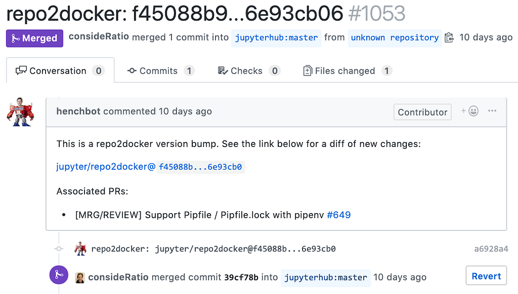
Here’s what we’re aiming for. The PR body:

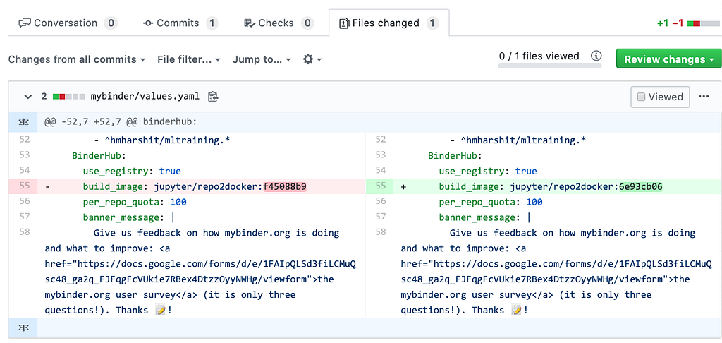
The PR diff:

Now that we’ve broken it down a bit, let’s write up some Python code. Once we have a functioning script, we can worry about how we will run this in the cloud (cron job vs. web app).

Writing the bot

If you don’t care about the step-by-step, you can skip to the final version of the code.

In the interest of linear understanding and simplicity for a bot-writing tutorial, the step-by-step below will not write functions or classes but just list the raw code necessary to carry out the tasks. The final version of the code linked above is one way to refactor it.

Step 1: Retrieve current deployed mybinder.org dependency versions

The first step is to see if any changes are necessary in the first place. Fortunately, @choldgraf had already made a script to do this.

To find the current live commit SHA for BinderHub in mybinder.org, we simply check the requirements.yaml file. We’ll need Python’s yaml and requests modules to make the GET request and parse the yaml in the response. Note that this is also conveniently the file we’d want to change to upgrade the version.

Similarly, for repo2docker, we check the mybinder.org values.yaml file:

Let’s store these SHAs in a dictionary we can use for later reference:

Step 2: Retrieve latest commits from the dependency repos

When we get the latest commit SHAs for repo2docker and BinderHub, we need to be careful and make sure we don’t automatically grab the latest one from GitHub. The travis build for mybinder.org looks for the repo2docker Docker image from DockerHub, and the latest BinderHub from the JupyterHub helm chart.

Let’s get the repo2docker version first:

Now we can do BinderHub:

Let’s add these to our dictionary too:

Great, now we should have all the information we need to determine whether an update needs to be made or not, and what the new commit SHA should be!

Step 3: Fork mybinder.org repo

If we determine an upgrade for the repo is necessary, we need to fork the mybinder.org repository, make the change, commit, push, and make a PR. Fortunately, the GitHub API has all the functionality we need! Let’s just make a fork first.

If you have permissions to a bunch of repos and organizations on GitHub, you may want to create a new account or organization so that you don’t accidentally start automating git commands through an account that has write access to so much, especially while developing and testing the bot. I created the henchbot account for this.

Once you know which account you want to be making the PRs with, you’ll need to create a personal access token from within that account. I’ve set this as an environment variable so it isn’t hard-coded in the script.

Using the API for a post request to the forks endpoint will fork the repo to your account. That’s it!

Step 4: Clone your fork

You should be quite used to this! We’ll use Python’s subprocess module to run all of our bash commands. We’ll need to run these within the for-loop above.

Let’s also cd into it and check out a new branch.

Step 5: Make the file changes

Now we need to edit the file like we would for an upgrade.

For repo2docker, we edit the same values.yaml file we checked above and replace the old SHA (“live”) with the “latest”.

For BinderHub, we edit the same requirements.yaml file we checked above and replace the old SHA (“live”) with the “latest”.

Step 6: Stage, commit, push

Now that we’ve edited the correct files, we can stage and commit the changes. We’ll make the commit message the name of the repo and the compare URL for the commit changes so people can see what has changed between versions for the dependency.

Awesome, we now have a fully updated fork ready to make a PR to the main repo!

Step 7: Make the body for the PR

We want the PR to have a nice comment explaining what’s happening and linking any helpful information so that the merger knows what they’re doing. We’ll note that this is a version bump and link the URL diff so it can be clicked to see what has changed.

Step 8: Make the PR

We can use the GitHub API to make a pull request by calling the pulls endpoint with the title, body, base, and head. We’ll use the nice body we formatted above, call the title the same as the commit message we made with the repo name and the two SHAs, and put the base as master and the head the name of our fork. Then we just make a POST request to the pulls endpoint of the main repo.

Step 9: Confirm and merge!

If we check the mybinder.org PRs, we would now see the automated PR from our account!

Step 10: Automating the script (cron)

Now that we have a script we can simply execute to create a PR ($ python henchbot.py), we want to make this as hands-off as possible. Generally we have two options: (1) set this script to be run as a cron job; (2) have a web app listener that gets pinged whenever a change is made and executes your script as a reaction to the ping.

Given that these aren’t super urgent updates that need to be made seconds or minutes after a repository update, we will go for the easier and less computationally-expensive option of cron.

If you aren’t familiar with cron, it’s simply a system program that will run whatever command you want at whatever time or time interval you want. For now, we’ve decided that we want to execute this script every hour.

Cron can be run on your local computer (though it would need to be continuously running) or a remote server. I’ve elected to throw it on my raspberry pi, which is always running. Since I have a few projects going on, I like to keep the cron jobs in a file.

$ vim crontab-jobs

You can define your cron jobs here with the correct syntax (space-separated). Check out this site for help with the crontab syntax. Since we want to run this every hour, we will set it to run on the 0 minutes, for every hour, every day, every month, every year. We also need to make sure it has the correct environment variable with the GitHub personal access token we created, so we’ll add that to the command.

0 * * * * cd /home/pi/projects/mybinder.org-upgrades && HENCHBOT_TOKEN='XXXXX' /home/pi/miniconda3/bin/python henchbot.py

Now we point our cron to the file we’ve created to load the jobs.

$ crontab crontab-jobs

To see our active crontab, we can list it:

$ crontab -l

That’s it! At the top of every hour, our bot will check to see if an update needs to be made, and if so, create a PR. To clean up files and handle existing PRs, in addition to some other details, I’ve written a few other functions. It is also implemented as a class with appropriate methods. You can check out the final code here.

Automating mybinder.org dependency upgrades in 10 steps was originally published in Jupyter Blog on Medium, where people are continuing the conversation by highlighting and responding to this story.

This is an invited post from Jim Colliander, Professor of Mathematics at UBC and Director of the Pacific Institute for the Mathematical Sciences.¹

In 2017, the Pacific Institute for the Mathematical Sciences (PIMS), in partnership with Compute Canada and Cybera, launched Syzygy, a cloud-hosted interactive computing platform that delivers JupyterHub deployments for universities across Canada.

Syzygy has been used by over 16,000 students at 20 universities. The main results of the Syzygy experiment so far are:

1. Demand for interactive computing is ubiquitous² and growing strongly at universities.
2. The Jupyter ecosystem is an effective way to deliver interactive computing.
3. A scalable, sustainable, and cost-effective interactive computing service for universities is needed as soon as possible.

Demand for interactive computing

Both research and teaching at universities are adapting to major societal changes driven by explosions in data and computational tools. New educational programs that prepare students to think computationally are emerging, while research strategies are changing in ways that are more open, reproducible, collaborative, and interdisciplinary. These transformations are inextricably linked and are accelerating demand for interactive computing. The Syzygy experiment has shown that using Jupyter in educational programs drives interest in using Jupyter for research (and vice versa). For example, students in mathematics, statistics, and computer science collaborated with a researcher from St. Paul’s Hospital in Vancouver using Syzygy to identify new pathways to prevent death from sepsis. Research communities typically need access to deeper computational resources and often span multiple universities, but the common thread is the need to expand access to interactive computing.

Technical milestone achieved

The Syzygy project has demonstrated that it’s possible to deploy tools for interactive computation at a national scale rapidly and efficiently using an entirely open source technology stack. Students, faculty and staff across Canada use Syzygy to access Jupyter through their browsers with their university single-sign-on credentials. The JupyterHubs range from a “standard” configuration to bespoke environments with specially curated tools and data integrations. This richness is possible because of the architecture of the Syzygy and Jupyter projects and the flexibility of the underlying cloud resources. As a case-study, Syzygy demonstrates that the Jupyter community has achieved a significant technical milestone: interactive computing can be delivered at national scale using cloud technologies.

Service level requirements

The validation that interactive computing can be technically delivered at national scale prompts universities to ask a variety of questions. Can interactive computing service be delivered robustly? How will users be supported? What are the uptime expectations? What is the data security policy? How is privacy protected? Can the robustness of the service be clarified in a service level agreement? Syzygy, as an experimental service offered to universities at no charge and without a service level agreement, does not properly address these questions. To advance on their education-research-service mission and address growing demand, universities need a reliable interactive computing service with a service level agreement.

What’s next?

How should universities address their needs for interactive computing over the next five years? Right now, universities are following two primary approaches:

• 🙏 Ad hoc: faculty figure out how to meet their own needs for interactive computing; IT staff deploys JupyterHub on local or commercial cloud servers; this approach gives universities control over their deployments and hardware, though requires time and expertise that many may not have.
• 🎩 Use a cloud provider’s service: Google Colab, Amazon Sagemaker, Microsoft Azure Notebooks, IBM Watson Studio; this approach allows universities to quickly launch interactive computing services, with a loss of flexibility and some risks by becoming reliant upon a particular vendor’s closed-source and proprietary software.

These approaches are not sustainable over the long term. If universities all deploy their own JupyterHub services, many will need technical expertise they do not currently have and will involve a significant duplication of effort. If universities rely on hosted cloud notebook services, the reliance on proprietary technology will impair their ability to switch between different cloud vendors, change hardware, customize software, etc. Vendor lock-in will limit the ability of universities to respond to changes in price for the service. Universities will lose agility in responding to changes in faculty, staff, and student computing needs.

There is a third option that addresses the issues with these two approaches and generates other benefits for universities:

• 🤔 Form an interactive computing consortium: universities collaborate to build an interactive computing service provider aligned with their missions to better serve their students, facilitate research, and avoid risks associated with vendor lock-in.

To retain control over their interactive computing stacks, avoid dependence⁴ on cloud providers, and accelerate the emergence of new programs, universities should work together to deploy interactive computing environments in a vendor-agnostic manner. This might take the form of a consortium — an organization dedicated to serving the needs of universities through customized shared infrastructure for interactive computing. The consortium would also ensure that universities will continue to play a leadership role in the development of the interactive computing tools used for education and research.

The Syzygy experiment confirmed that growing demand for interactive computation within universities can be supplied with the available technologies advanced by the Jupyter open source community. In the coming year, we aim to build upon the success of the Syzygy experiment and seed an initial node of a consortium in Canada with the intention of fostering a global network of people invested in advanced interactive computing. If you are interesting in partnering, please get in touch! See this Jupyter Community Forum post to continue the discussion.

1. The author gratefully acknowledges feedback on this piece from Ian Allison, Lindsey Heagy, Chris Holdgraf, Fernando Perez, and Lindsay Sill.
2. Interactive computing needs have been identified in agriculture, applied mathematics, astronomy, chemistry, climate science, computer science, data science, digital humanities, ecology, economics, engineering, genomics, geoscience, health sciences, K-12 education, neuroscience, political science, physics, pure mathematics, statistics, and sociology.
3. Relying on commercial cloud vendors to provide the interactive computing service for universities risks recreating the problems associated with scientific publishing that emerged with the internet.

National Scale Interactive Computing was originally published in Jupyter Blog on Medium, where people are continuing the conversation by highlighting and responding to this story.

By Lindsey Heagy and Fernando Pérez

We are thrilled to announce that the NSF is funding our EarthCube proposal “Jupyter meets the Earth: Enabling discovery in geoscience through interactive computing at scale” (pdf). The team working on this project consists of Fernando Pérez [1, 2, 3], Joe Hamman [4], Laurel Larsen [5], Kevin Paul [6], Lindsey Heagy [1], Chris Holdgraf [1, 2] and Yuvi Panda [7]. Our project team includes members from the Jupyter and Pangeo communities, with representation across the geosciences including climate modeling, water resource applications, and geophysics. Three active research projects, one in each domain, will motivate developments in the Jupyter and Pangeo ecosystems. Each of these research applications demonstrates aspects of a research workflow which requires scalable, interactive computational tools.

In this project we intend to follow the patterns that have made Jupyter an effective and successful platform: we will drive the development of computational machinery by concrete use cases from our own experience and research needs, and then find the appropriate points for extension, abstraction, and generalization. We are motivated to advancing research of contemporary importance in geoscience, and are equally committed to producing work that leads to broad impact, general use infrastructure that benefits scientists, educators, industry, and the general community.

The adoption of open languages such as Python and the coalescence of communities of practice around open-source tools, is visible in nearly every domain of science. This is a fundamental shift in how science is conducted and shared. In recent years, there have been several high-profile examples in which open tools from the Python and Jupyter ecosystems played an integral role in the research, from data analysis to the dissemination of results. These include the first image of a black hole from the Event Horizon Telescope team and the detection of gravitational waves by the LIGO collaboration. The utility of open-source software in projects like these and the success of open communities such as Pangeo, provide evidence of the force-multiplying impact of investing in an ecosystem of open, community-driven tools. Through this project, we will advance this open paradigm in geoscience research, while strengthening and improving the infrastructure that supports it. We made this argument when discussing the intended impacts of our proposal, and we are pleased that the NSF is investing in this vision.

Geoscience use cases

Given our project’s aims and approach, participating actively in domain research is crucial to our success. The following descriptions are meant to offer a flavour of the research questions we are tackling, each led by a geoscientist in the team.

CMIP6 climate data analysis (Hamman). The World Climate Research Program’s Coupled Model Intercomparison Project is now in its sixth phase and is expected to provide the most comprehensive and robust projections of future climate predictions. When complete, the archive is expected to exceed 18 PB in size. In the coming years, this collection of climate model experiments will form the basis for fundamental research, climate adaptation studies, and policy initiatives. While the CMIP6 dataset is likely to hold new answers to many pressing climate questions, the sheer volume of data is likely to present significant challenges to researchers. Indeed, new tools for scalable data analysis, machine learning, and inference are required to make the most out of these data.

Large-Scale Hydrologic Modeling (Larsen). Streamflow forecasts are a valuable tool for flood mitigation and water management. Creating these forecasts requires that a variety of data types be brought together including model-generated streamflow estimates, sensor-based observations of water discharge, and hydrometeorological forcing factors, such as precipitation, temperature, relative humidity, and snow-water equivalent. The integration of simulated and observed data over disparate spatial and temporal scales creates new avenues for exploring data science techniques for effective water management.

Geophysical inversions (Heagy). Geophysical inversions construct models of the subsurface by combining simulations of the governing physics with optimization techniques. These models are critical tools for locating and managing natural resources, such as groundwater, or for assessing the risk from natural hazards, such as volcanoes. Today, we need models applicable to increasingly complex scenarios, such as the socially delicate task of developing groundwater management policies in water-limited regions. This will require the development of new techniques for combining multiple geophysical data sets in a joint inversion, as well as the use of statistical and data science methods for including geologic and hydrologic data in the construction of 3D models.

These scientific problems exhibit, each with its own flavour, similar technical challenges with respect to handling large volumes of data, performing expensive computations, and doing both of these as a part of the interactive, exploratory workflow that is necessary for scientific discovery.

Jupyter & Pangeo: empowering scientists

Jupyter and Pangeo are both open communities that share the goal of developing tools and practices for interactive scientific workflows; these tools aim to deliver practical value to scientists who, in the course of everyday research, face a combination of big data and large-scale computing needs.

Project Jupyter creates open-source tools and standards for interactive computing. These span the spectrum from low-level protocols for running code interactively up to the web-based JupyterLab interface that a researcher uses. Jupyter is agnostic of programming language: over 130 different Jupyter kernels exist, and they provide support for most programming languages in widespread use today. Jupyter can be run on a laptop, in an HPC center, or in the cloud. Shared-infrastructure deployments (e.g. HPC / cloud) are enabled by JupyterHub, a component in the Jupyter toolbox that supports the deployment and management of Jupyter sessions for multiple users. The development process of tools in the Jupyter ecosystem is community-oriented and includes a diverse set of stakeholders across research, education, and industry. The project has a strong tradition of building tools that are first designed to solve specific problems, and then generalized to other users and applications.

A Pangeo Platform is a modular composition of open, community-driven projects, tailored to the scientific needs of a specific scientific domain. In its simplest form, it is based on the following generic components: a browser-based user interface (Jupyter), a data model and analytics toolkit (Xarray), a parallel job distribution system (Dask), a resource management system (either Kubernetes or a job queuing system such as PBS), and a storage system (either cloud object store or traditional HPC file system). These are complemented by problem- and domain-specific libraries.

This modular design allows for individual components to be readily exchanged and the system to be applied in new use cases. Pangeo was created by, and for, geoscientists faced with large-scale data and computation challenges, but such problems are now common in science. Researchers in a variety of disciplines including neuroscience and astrophysics are working to adapt the Pangeo design pattern for their communities. Beyond the initial Pangeo deployments supported by the NSF EarthCube grant for Pangeo, the platform has been adopted internationally, including by the UK Met office. It has also supported new research and education efforts from other federal agencies, such as NASA’s HackWeek focused on the analysis of ICESat-2 data.

User-Centered Development

Pushing the boundaries of any toolset unveils areas for improvement and opportunities for developments that streamline and upgrade the user experience. We aim to take a holistic view of the scientific discovery process, from initial data acquisition through computational analysis to the dissemination of findings. Our development efforts will make technological improvements within the Jupyter and Pangeo ecosystems in order to reduce pain-points along the discovery lifecycle and to advance the infrastructure that serves scientists. Following established patterns in Jupyter’s development, we take a user-first, needs-driven approach and then generalize these ideas to work across related fields. Broadly, there are 4 areas along the research lifecycle where we will invest development efforts, which we discuss next.

Data discovery. An early step in the research process is locating and acquiring data of interest. Data catalogs provide a way to expose datasets to the community in a way that is structured. Within the geosciences, there are a number of emerging community standards for data catalogs (e.g. THREDDS, STAC). To streamline access to such data sets, we plan to develop JupyterLab extensions which provide a user-interface that exposes these catalogs to researchers. This work will build upon the JupyterLab Data Registry, which will provide a consistent set of standards for how data can be consumed and displayed by extensions in the Jupyter ecosystem, as well as Intake, a lightweight library for finding, loading, and sharing data which is already serving the Pangeo community. Our communities are already discussing potential avenues for integration between these tools.

Scientific discovery through interactive computing. The Jupyter Notebook has been adopted by many scientists because it supports an iterative, exploratory workflow combining code and narrative. Beyond code, text, and images, Jupyter supports the creation of Graphical User Interfaces (GUIs) with minimal programming effort on the part of the scientist. The Jupyter widgets framework lets scientists create a “Research GUI” that combines scientific code with interactive elements such as sliders, buttons and menus in just a single line of code, while still allowing for extensive customization and more complex interfaces when required. In this project, we will develop custom widgets tailored at the specific scientific needs of each of our driving use cases.

Beyond their utility in the exploratory phase of research, interactive interfaces, or “dashboards” provide a mechanism for delivering custom scientific displays to collaborators, stakeholders, and students for whom the details of the code may not be pertinent. Voilà is a project, led by the QuantStack team, that enables dashboards to be generated from Jupyter notebooks. We plan to develop interactive dashboards using Voilà for our geoscience use-cases, contribute generic improvements to the Voilà codebase, and provide a demonstration of how researchers can deploy dashboards to share their research.

Established tools and data visualization. Many widely-used tools, particularly for visualization (e.g. Ncview, Paraview), are desktop-based applications and therefore cannot easily be used in cloud or HPC workflows. In some cases, modern, open-source alternatives are available. But often for specialized tasks, modern tools may not yet have functionality equivalent to the desktop version. JupyterHub can readily serve non-Jupyter web-native software applications such as RStudio, Shiny applications, and Stencila to users; under this project we aim to extend JupyterHub to also be able to serve desktop-native applications.

Using and managing shared computational infrastructure. JupyterHub makes it possible to manage computing resources, user accounts, and provide access to computational environments online. Currently, JupyterHubs in the Pangeo project are deployed and maintained using the Zero to JupyterHub guide alongside the HubPloy library. Together, these libraries have simplified the initial setup and automated upgrades to the Hubs. There are still many improvements that can make JupyterHub more suitable for larger, more complex deployments, both in terms of managing users and efficiently allocating resources. Under this project, we plan to build tools which collect metrics such as CPU and memory usage and expose these to both users and administrators so they can make more efficient use of the Hub. For shared deployments, we will improve user management so that user-groups can be used to manage permissions and allocations, and so that usage can be tracked and appropriately billed to the relevant grants. Within the HubPloy library, we also plan to make improvements to streamline continuous deployments so that installation and upgrade processes are repeatable and reliable.

An opportunity for meaningful impact — join us!

The impacts of climate change and the need for data-driven management of resources are some of the most critical and complex challenges facing society today. In recent years, we have experienced severe droughts in California and are in the midst of water management crises in the Central Valley, while devastating wildfires have destroyed entire communities. Through this partnership between researchers and Jupyter developers, we hope to contribute to the advancement of science-based solutions to these challenges, both by contributing directly to the research and by improving the open ecosystem of tools available to researchers and the stakeholders impacted by these issues.

If developing open-source tech to advance research in geoscience and beyond excites you, then please get in touch! At UC Berkeley, we will be hiring in 2 positions: a dev-ops position focussed on JupyterHub and shared infrastructure deployments, and a JupyterLab-oriented role focussed on extensions, dashboards, and interactivity. There will also be a position opening up at NCAR for a software engineer targeting improvements to improving the user experience of Xarray and Dask workflows.

Even if you aren’t looking for a new job, there are other ways to get involved with both the Jupyter and Pangeo communities. We welcome new participants to the weekly Pangeo meetings (on Wednesdays alternating between 4p GMT and 8p GMT) and there are monthly Jupyter community calls, which are open and meant to be accessible to a wide audience. Outside of calls, general Jupyter conversations happen on the Jupyter discourse and Pangeo conversations are typically on the Pangeo GitHub.

In closing: a step toward sustainable open science

This project provides our team with $2 Million in funding over 3 years as a part of the NSF EarthCube program. It also represents the first time federal funding is being allocated for the development of core Jupyter infrastructure.

The open source ecosystem that Jupyter and Pangeo belong to has become part of the backbone that supports much of today’s computation in science, from astronomy and cosmology to microbiology and subatomic physics. Such broad usage represents a victory for this open and collaborative model of building scientific tools. Much of this success has come through the efforts of scientists and engineers who are committed to an open model of science, but who have had to work with little direct funding, minimal institutional support, and few viable career paths within science.

There is real strategic risk to continuing with the implicit assumption that scientific open-source tools can be developed and maintained “for free.” If open, community-driven tools are to sustainably grow into the computational backbone of science, we need to recognize this role and support those who create them as regular members of the scientific community (we recently talked about this in more detail in a talk at NSF headquarters). Projects like ours, where funding and resources are explicitly allocated toward this goal, are a step in the right direction. We hope that our experiences will contribute to ongoing conversations in the scientific community around these complex issues.

In the past, we have tried to maintain a close relationship between domain problems and software development in Jupyter. However, this has typically been done in an ad-hoc manner, either by “hiding” the software development under the cover of science or by having funding to Jupyter alone. This is the first project where we explicitly partner with a team of domain scientists to simultaneously drive forward domain research and the development of Jupyter infrastructure.

We are excited about this opportunity and hope to be able to demonstrate that investing in open tools can be a force-multiplier of resources. As always, our work will be done openly, transparently, and with constant community engagement. We look forward to your critiques, ideas, and contributions to make this effort as successful as possible.

Acknowledgments

Thanks to Joe Hamman, Chris Holdgraf, and Doug Oldenburg for constructive feedback and edits on this blog post.

Many thanks to Ryan Abernathey (Columbia), Paul Bedrosian (USGS), Sylvain Corlay (QuantStack), Rich Signell (USGS), and Rollin Thomas (NERSC), who provided us with letters of support for this project; we look forward to working with you all! We are also grateful to Shree Mishra, our NSF Program Director on this project, and to Dave Stuart for their support as we move forward with the project. This project is a part of the to the EarthCube program and we look forward to engaging with its working group.

Finally, the sustained growth of Jupyter to the large-scale project that it has become would not have happened without the generous support of the Alfred P. Sloan, the Gordon and Betty Moore, and the Helmsley Foundations, as well as the leadership of Josh Greenberg and Chris Mentzel respectively at Sloan and Moore.

Affiliations

[1] UC Berkeley, Statistics Department

[2] UC Berkeley, Berkeley Institute for Data Science

[3] Lawrence Berkeley National Lab, Computational Research Division

[4] National Center for Atmospheric Research, Climate and Global Dynamics Laboratory

[5] UC Berkeley, Department of Geography

[6] National Center for Atmospheric Research, Computational Information Systems Laboratory

[7] UC Berkeley, Division of Data Sciences

Jupyter meets the Earth was originally published in Jupyter Blog on Medium, where people are continuing the conversation by highlighting and responding to this story.

As Jupyter grew in popularity, a broad ecosystem of visualization packages based on Jupyter widgets has been developed, bringing even more interactivity to the Jupyter world.

In this article, we dive into Jupyter Interactive Widgets and the ipyleaflet package, an interactive maps visualization system for Jupyter.

Jupyter Widgets

Jupyter Interactive Widgets are “special objects” that can be instantiated by the user in their code and result in a counterpart component being created in the front-end.

The core ipywidgets package provides a collection of controls that Jupyter users can use to build simple UIs as part of their notebooks (sliders, buttons, dropdowns, layout components).

More than a collection of controls, it provides a framework upon which a large ecosystem of components has been built, allowing notebook authors to capture user inputs in very diverse ways.

Popular libraries built upon interactive widgets include

• bqplot, a 2-D plotting system for Jupyter,
• ipyvolume, a 3-D plotting package based on WebGL and ThreeJS,
• PythreeJS, a 3-D scene description package exposing a large part of the ThreeJS API to Jupyter,
• ipyvuetify, a large collection of VuetifyJS components exposed to Jupyter,
• ipywebrtc, a library exposing the features of the WebRTC protocol to Jupyter kernels,
• beakerx, a collection of widgets, extensions, and kernels for Jupyter,

and many more… This list is not comprehensive and dozens of other widget packages have been developed.

Key aspects of Jupyter widgets include:

• Bidirectionality
  Widgets are not just meant for display but can also be used to capture user inputs, which can then trigger new computation. Notebook authors can compose sophisticated applications including a variety of components from different packages.
• Language Agnosticism
  Built upon the Jupyter ecosystem, the interactive widget protocol used for the synchronization between the kernel and the front-end is well-specified and can be implemented for any kernel.
  Back-ends for other languages than Python already exist, such as for C++ (with the xeus-cling Jupyter kernel), and languages of the JVM such as Clojure or Groovy (with the beakerx kernels).
• Extensibility
  Jupyter widgets are not meant as a monolithic system with one and only one way to achieve a specific task. We strive to provide a foundational layer allowing third-party widget authors to be as inventive as possible.

A common pattern for Jupyter widget packages has been to bring the capabilities of popular JavaScript visualization frameworks to Jupyter with a bridge based on ipywidgets. This is the case for the ipyleaflet package, as well as pythreejs and ipyvuetify.

Another use case is the development of ad hoc controls that are not necessarily relevant for a mainstream visualization package, but may be specific to a scientific field. An example is the ipymesh project by Chris Kees which can be used to draw PSLG (planar straight-line graphs) in the Jupyter notebook.

ipyleaflet

ipyleaflet is a Jupyter - LeafletJS bridge, bringing mapping capabilities to the notebook and JupyterLab.

Built as a bridge between the LeafletJS package and Jupyter, the ipyleaflet API maps to that of LeafletJS, bringing most of the core features of the package to Jupyter, and enabling a few popular LeafletJS extensions. A small difference is that following the Python coding style, ipyleaflet makes use of snake_case instead of CamelCase for attribute names.

ipyleaflet features

The main components to the library are layers and controls, respectively items to be displayed on the map, and interactive widgets overlayed on the map area for greater interactivity.

The first thing for which you may want to change the default value are the zoom level, the position, or the base layer for the map.

Maps can be interactively edited in the Jupyter notebook, by dynamically changing or adding layers. In this screenshot, we add a custom layer including a GeoJSON dataset.

Note: An alternative layer to GeoJSON is GeoData, which lets the user load the data in the form of a GeoPandas dataframe instead of raw GeoJSON.

A number of simple primitives are available such as markers and heatmaps. In the following screencast, we show how primitive properties can be linked with other widgets, and used as means to take user input on a map:

The splitmap control can be used to compare to different set of ipyleaflet layers at the same location.

Another interesting layer is the velocity layer which can be used to display wind velocity data. This control can take data in the form of an xarray dataset.

More classical visualization tools are also available, such as choropleths.

JupyterLab Integration with the Sidecar and Theming Support

ipyleaflet is well integrated with JupyterLab

• ipyleaflet controls make use of the JupyterLab themes for coloring so that they don't stand out when using e.g. a dark theme.

• ipyleaflet can be used in combination with the JupyterLab sidecar widget.

Together with the sidecar, a map can be programmatically added to the right-side toolbar of the JupyterLab application, and interactively edited in the notebook. This prevents the back-and-forth scrolling often required to see how changes are reflected visually.

The workflow enabled by ipyleaflet in combination with the sidecar is similar to that of the geonotebook project by Christopher Kotfila, Jonathan Beezley, and Dan LaManna from Kitware).

A more advanced example

Combined with other widget libraries such as bqplot or the core ipywidget package, ipyleaflet users can easily compose more complex applications and dashboards. In the following screencast, we explore the wealth-of-nations dataset with a leafletmap, a bqplot line chart and a dropdown widget:

Trying ipyleaflet online with mybinder

If you would like to try out ipyleaflet now, it is possible thanks to the binder project. Just click on the image below!

Interactive GIS in C++: xleaflet

As mentioned earlier, interactive widgets back-ends for other programming languages have be implemented. There is a C++ back-end for ipywidgets: xwidgets which is the building block for creating other C++ widgets back-ends.

xleaflet is the C++ - LeafletJS bridge that exposes almost the same API as ipyleaflet, only that you use it from a C++ interpreter! It is based upon xwidgets which brings the bidirectional communication with the front-end.

You can learn more about the xeus-cling Jupyter kernel, xwidgets and xleaflet by reading the following blogpost.

Deploying ipyleaflet-based dashboards with Voilà

Voilà is a tool that turns Jupyter notebooks into standalone dashboards. Built upon the Jupyter stack, it inherits the language agnosticism of the ecosystem, and can be used to produce standalone applications based on ipyleaflet.

A companion project to Voilà is the Voilà gallery project, a public facing set up of JupyterHub serving Voilà dashboard. It is kindly hosted by OVH. You can check out the Voilà gallery at URL https://voila-gallery.org.

For more resources about voilà, check out

• the original announcement of the project: And Voilà!
• and for the gallery: A Gallery of Voilà Examples.

If you check out the Voilà gallery, don't miss Jeremy Tuloup's GPX loader demo!

Jupyter for Geo Sciences

Jupyter's adoption is exploding in the GeoScience space. Notable projects building upon Jupyter include

• JEODPP (JRC Earth Observation Data and Processing Platform) is a EU project providing petabyte scale storage and high-throughput computing capacities to facilitate large scale analysis of Earth Observation data. The main front-end to the platform is base on Jupyter. The mapping capability is based on ipyleaflet. End users can request custom visualization that are returned to them in the form of lazily computed tile layers.
• Pangeo is a community platform providing open, reproducible, and scalable sciences. The Pangeo software ecosystem involves open source tools such as xarray, Iris, Dask, Jupyter, and many other packages.
• It was recently announced that the NSF would be funding the UC Berkeley + NCAR "EarthCube" proposal "Jupyter meets the Earth: Enabling discovery in geoscience through interactive computing at scale". The plan involves the development of interactive dashboards with Voilà and contributions to the Voilà codebase.

Related Projects

Jupyter-gmaps

We should mention the jupyter-gmaps project by Pascal Bugnion. Jupyter-gmaps is a bridge between Google maps and Jupyter. Just like ipyleaflet, jupyter-gmaps is built upon the jupyter interactive widgets framework but relies on Google maps for the display instead of LeafletJS library.

This is a high-quality widget by another core developer of ipywidgets. Pascal is also one of the people behind Voilà and the Voilà gallery.

Folium

The Folium project enables maps visualization in the Jupyter notebook. Just like ipyleaflet, it is based on LeafletJS. Folium was created by Rob Story and is now maintained by Frank Conengmo and Filipe Fernandes.

A key difference between Folium and ipyleaflet is that ipyleaflet is built upon ipywidgets and allows bidirectional communication between the front-end and the backend enabling the use of the map to capture user input, while Folium is meant for displaying static data only. Folium enables many LeafletJS extensions, some of which may not be available in ipyleaflet at the moment.

Acknowledgements

The ipyleaflet project was started in 2015 by Brian Granger, and funded by the ERDC. The further development by Sylvain Corlay and Martin Renou was supported by QuantStack.

We are grateful to OVH for kindly hosting the Voilà gallery.

Other key contributors to Voilà and ipyleaflet that should be thanked here are Maarten Breddels, Pascal Bugnion, and Yuvi Panda. We should also mention the recent contributions by Vasavan Thirusittampalam who worked on the full-screen control and better interoperability with geopandas.

About the Authors

Sylvain Corlay, and Martin Renou are Scientific Software Developers at QuantStack.

Sylvain Corlay

Sylvain Corlay is the founder and CEO of QuantStack.

As an Open Source Developer, Sylvain contributes to Project Jupyter in the areas of interactive widgets and language kernels and is a steering committee member of the Project. Beyond QuantStack, Sylvain serves as a member of the board of directors of the NumFOCUS foundation. He also co-organizes the PyData Paris Meetup.

Martin Renou

Martin Renou is a Scientific Software Developer at QuantStack. Prior to joining QuantStack, Martin also worked as a Software developer at Enthought. He studied at the French Aerospace Engineering School ISAE-Supaero, with major in autonomous systems and programming.

As an open source developer, Martin has worked on a variety of projects, such as SciviJS (a JavaScript 3-D mesh visualization library), Xtensor, and Xeus.

Interactive GIS in Jupyter with ipyleaflet was originally published in Jupyter Blog on Medium, where people are continuing the conversation by highlighting and responding to this story.

Earlier this summer a workshop to gather the Jupyter community in South America was held in Córdoba, Argentina, from Jun 22nd to Jun 23rd, 2019. We enjoyed the participation of contributors from different regions of Argentina, Chile, and Venezuela.

The workshop consisted of several hands-on discussions, hacking sessions, and some quick presentations showing off the work done during the hacking time.

Attendees were able to contribute to several areas of the Jupyter ecosystem. There was particular interest in JupyterLab, Jupyter in Education (at different stages with its own particularities), discussions about some core Jupyter building blocks and some remarkable work on beginning the translation of documentation to Spanish.

To keep the group in sync, to have discussions and to build new things, we created a group in telegram which we invite you to check out: https://t.me/jupyter_latam. Everyone is welcome to participate! Join us!

Why organize a workshop for South American contributors?

The main driving idea was to conglomerate (and foster) a group of people interested in the Jupyter ecosystem, plant some seeds and spread the interest across the regions the attendees came from.

The Jupyter community is the vital force that builds and sustains the Jupyter ecosystem.

We were also interested in increasing the diversity of our current Jupyter community - bringing not only new ideas but also new Jupyter developments and solutions to solve some of the problems we see in South America.

What did the attendees get from the event?

We got to know each other, we kick off some interesting discussion and conversations, we helped each other to understand some of the particularities of the Jupyter ecosystem and we brainstormed future steps for this group’s point of view and how it could help the whole Jupyter community.

In the midst of all this activity we also had fun! We hacked together, we solved problems and found new questions, we were inspired to continue contributing, we got more experienced about Jupyter tools, and we leveraged each others expertise to build new and exciting things.

In summary, a wonderful experience ;-)

What’s happening next?

We discussed the pros and cons of the event format and how could eventually replicate the experience in other parts of South America. Stay tuned for news about the upcoming events in the future!

Acknowledgments

This event would not have been possible without the generous financial support provided by Bloomberg.

Many thanks to Lisa Martin and Lynn Brubaker (from NumFocus) and Ana Ruvalcaba from Project Jupyter for their help and advice. I would also like to thank my co-organizer, Daniela Bermejo, for her endless help in all the tasks related to the event organization.

Finally, I would like to offer a sincere thank you to all the attendees who shared their personal time to come together to help create a community with a wonderful future.

South America Jupyter Community Workshop was originally published in Jupyter Blog on Medium, where people are continuing the conversation by highlighting and responding to this story.

From May 27th to May 29th, thirty developers from the Jupyter community met in Paris for a three-days workshop on the Jupyter kernel protocol.

For three days, attendees worked full time on the Jupyter project, including hacking sessions and discussions on improvements to Jupyter protocols and standards.

We were lucky to count five core developers to the project and several more regular contributors to the larger ecosystem in the group!

Beyond the hacking session, each day was concluded with a series of presentations and demos of the progress made during the workshop.

Why a workshop on Jupyter kernels?

The Jupyter Kernel protocol is one of the main extension points of the Jupyter ecosystem. Dozen of language kernels have been developed by the community, and these languages can then leverage the other components of the stack, such as the notebook, the console, and interactive widgets.

One of the objectives of this event was to foster collaboration between kernel developers and core contributors and develop common tools used across all language kernels. Another goal was to work improving the protocol, to support visual debugging, parameterized kernels, etc.

Technical Achievements

A lot of work was done during the workshop. Several people were working on new Jupyter kernels for programming languages.

We were amazed to see how much was achieved in just three days. Today, we are still working on projects that stemmed from this community workshop.

JupyterLab Debugger

One area in which the Jupyter team is actively working is support for visual debugging in JupyterLab. This is a major endeavor spanning from the front-end to the back-end, including changes to the Jupyter protocol.

The kernel workshop was the occasion for several developers (Wolf Vollprecht, Maarten Breddels, Johan Mabille, Loic Gouarin) to get together and hack on the implementation of the frontend. A lot of work had been done ahead of the workshop with a new Python kernel based on the Xeus library. This new kernel includes a backend to the Debug Adapter Protocol over kernel messages.

There are other key contributors to the debugger project who did not attend the community workshop. We should mention Jeremy Tuloup and Afshin Darian who are spearheading the frontend development.

A Calculator Jupyter Kernel based on xeus

Vasavan Thirusittampalam and Thibault Lacharme were in the middle of their summer internships as scientific software developers at QuantStack when they attended the workshop. During the event, they set themselves up to implement a new Jupyter kernel in C++!

At the end of the workshop, they were able to demonstrate a functional calculator kernel based on xeus, a C++ implementation of the Jupyter protocol! This was later polished and resulted in the publication of a blog post on the Jupyter blog: "Building a Calculator Jupyter Kernel". This example may serve as an example for people interested in creating new language kernels with xeus.

A prototype Julia backend to Jupyter interactive Widgets.

During the workshop Sebastian Gutsche (who is the author of the Singular Jupyter kernel and a co-author of the GAP kernel), set himself to develop a backend to Jupyter interactive widgets for the Julia progamming language. The current state of the code can be found here.

The Julia backend to jupyter widgets is still early-stage but should this project be completed, it would enable other Jupyter widget libraries for the users of the Julia Jupyter kernel, such as ipyvolume, ipyleaflet, bqplot, etc.

Parameterized Kernelspecs

Paul Ivanov and Kyle Kelley worked on ironing out the proposal for the support of parameterized kernelspecs. The objective is to make it possible to pass user-specified arguments to kernels upon launch.

In the proposal, the parameters expected by the kernel executable and the possible values for these parameters may be specified in the kernelspec file or a companion file to the kernelspec in the form of a JSON schema.

Paul and Kyle produced extensive notes on various aspects on the subjects such as

• the storing of previously used values of the parameters (in notebooks)
• the web UI design on how to specify parameters
• the definition of default values

More details will be shared at a later stage on the subject of parameterized kernelspecs.

Note: the subject of parameterized kernelspecs was also central in the earlier community workshop about the Jupyter server organized at IBM by Luciano Resende.

Forking of Jupyter Kernels

Starting of kernels is an expensive operation, and executing a whole notebook even more. For certain use cases (such as dashboards based on Voilà), it is useful to have a pre-executed notebook ready, so that dashboards can be presented instantly to a user. To enable this, Maarten Breddels came up with the idea of forking kernels and put together a proof-of-concept implementation. The implementation can be found in pull requests to jupyter_client (PR #441) and ipykernel (PR #410).

Forking kernels will also allow interesting features such as an undo/rollback of cell execution in the notebook. While it is still a proof of concept, this subject has already sparked interest in the community.

Acknowledgments

This event would not have been possible without the generous support provided by Bloomberg, who made this workshop series possible

We are grateful to CFM for gracefully hosting the event.

We should also thank Ana Ruvalcaba from Project Jupyter for her incredible work on the logistics and finances of the Jupyter Community Workshop series.

Field Report on the Kernel Community Workshop was originally published in Jupyter Blog on Medium, where people are continuing the conversation by highlighting and responding to this story.